Greetings! In this activity, the ability to segment specific objects in an image will be discussed. There are many ways in order to segment an image such as thresholding methods, color-based segmentation, transform methods, and texture methods. (This is a link to the different types of segmentation: https://www.mathworks.com/discovery/image-segmentation.html).
We start off with grayscale thresholding and the provided image below will be used for this part of the activity.

Taking the grayscale histogram values of the image there exists a noticeable peak in the plot:

This peak corresponds to the values that are mostly present in the image… the background. In order to only segment the written text in the image, the gray values that are not part of the peak should be included therefore we start by thresholding at the value of 150 which give us..

Wow, the image segmented the written text! We are basically done but lets do two more just for good measure. threshold values are 130 and 110 for these:


Done! Now we move to color segmentation but let me discuss the mathematical background of color segmentation before we continue to the fun parts.
Normalized chromacity coordinates (NCC)!! Do not forget this three words. This is just a color space where the different rgb values of a pixel are represented. The equations of this space are derived below:
I = R+G+B
r = R/I; g = G/I; b = B/I
Clearly it can be seen that r + g + b = 1. Therefore we only need to plot two variables in order to express all possible rgb combinations in NCC(red and green. it depends actually but this is the standard for NCC). The NCC color space for red and green is shown below:

There! Now its a little bit easier to segment objects that are not in grayscale. This is important because shading variations not only show brightness but also how it affects color.
I. Parametric Probability Distribution
In this color segmentation technique, we segment by comparing if a pixel belongs to a color distribution (in this case a gaussian distribution). We can then think of these distributions as probability distribution functions. Combining this with the knowledge we know about the NCC, we only need the probability distribution of red and green, p(r) and p(g). The probability distributions are shown below:

The joint probability of these equations P = p(r)p(g) determines if a pixel belongs to a region of interest. Let us move to the fun part. Below is the image to be used for this activity.


The image on the right is the region of interest (ROI) which comes from cutting a square in the middle of the red ball. The mean and the standard deviation of the region of interest is found out and used in the calculation of the joint probabilities to compare each pixel membership. This gives the segmented image:

In order to improve on the quality of segmentation, better ROI’s are needed.
II. Non-parametric Segmentation
This differs from the earlier technique because we will be using histogram backprojection. Each pixel is translated to it’s histogram value in NCC. Taking the histogram values of the ROI earlier will give the histogram values for pixel membership…

And so using this technique the segmented image looks like this:

In comparing this image to the parametric segmentation, it can be seen that parametric segmentation is better for this picture. But of course both methods gives a segmented image by color. I believe that a clear difference in the methods are a smoother shade variation is seen in parametric segmentation than non-parametric segmentation. This makes sense because we assumed a continuous probability distribution function for the parametric segementation.
Phew.. unto more adventures.
I would like to thank Kit and Roland for useful insights.

Leave a comment