Area Estimation

Green’s Theorem in Discrete form

First and foremost, Green’s theorem is a vector identity which relates the line integral of a closed curve and it’s area inside the curve. This is mostly used in electrodynamics ( as far as I’ve remembered. This activity focuses on area and length estimation in images using the discrete form of the greens function. In integral form the area enclosed in a curve is given by,

$latex A = \int_{0}^{1} (xy^{‘} – yx^{‘})dt $

and considering that the image is formed by discrete pixels the equation becomes,

$latex A = \sum_{0}^{1} (xy^{‘} – yx^{‘}) $

This equation will be used in order to estimate the area of any 2d space in an image. We treat the area to be estimated with the value of 1 and 0 for the values we do not wish to measure. In order to know the bounds of the image,  the edges are important to consider.

In this exercise, I focused more on “prewitt” edge detection in scilab. I also simulated the accuracy of the edge detection by changing the pixel count of the NxN grid of three shapes namely a square, a circle, and a triangle. For the first part of the activity I simulated the shapes with varying pixel count but not changing the ratio of the shape with the size of the grid. This method changes the resolution of the image but not the area of the shape.

A circle

A Square

A Triangle

I started from a 100×100 grid and increasing the size by 20×20. I want to show the edges detected by using the edge module of SciLab first. The pictures below corresponds to the edges of the shapes above.

Edges of Circle

Edges of a Square

Edges of a Triangle

After taking the edges, the center of the shape is needed in order to sort the coordinates of the edges from the angle coming form the center. Once this is done, the discrete greens function can be used to calculate the Area within the edges. The code below shows the entire procedure.

---

for S = 1:length(Shapes)

[x,y] = find(Shapes(S));

xcent = round(sum(x)/length(x));
ycent = round(sum(y)/length(y));
x = x-xcent;
y = y-ycent;

r = sqrt(x.^2 + y.^2);
theta = atan(y,x);

[thetainc , i] = gsort(theta,'g','i');

sortx = x(i);
sorty = y(i);

A = 0;

for i = 1:length(sortx)-1
 A = A + sortx(i)*sorty(i+1) - sorty(i)*sortx(i+1);
end

A = A* 1/2.;
if S==1
deviation1 = [deviation1 abs(A-theo(S))/theo(S)*100]
end
if S==2
deviation2 = [deviation2 abs(A-theo(S))/theo(S)*100]
end
if S==3
deviation3 = [deviation3 abs(A-theo(S))/theo(S)*100]
end
end

---

 

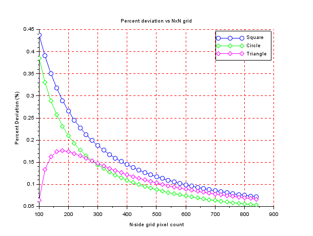
As seen in the code above, The input of the loop are the edges of the three shapes. What I wanted to show next is the accuracy of the prewitt edge detection algorithm. This is why the percent deviation of the number of pixels inside the edges are calculate. The theoretical values used are the number of pixels of the shape itself. The plot below shows the accuracy vs the size of the grid (essentially the resolution).

You may have noticed that the Square and the Circle have slightly similar trend lines. This may be because when a circle is created using smaller grids it will tend look more like a square (you can try this by creating a circle using 4×4 grid). Although, all shapes are accurate when you increase the resolution of the image.

Now that we know the accuracy of the prewitt edge detection scheme, we move to real world applications of this technique in estimating the area of a building. The photo below is a cropped image from google maps showing SM Olongapo. This is where i spent most of my childhood playing games and asking for toys (gone are the days). Anyway here it is,

 

SM Olongapo

 

I’ve marked the area of interest using this website: Daft Logic: Area calc. . From this site, the area of the highlighted region will show the area precisely. The area of the region is 5832.12 m². I believe that this sight is also using edge detection techniques to estimate the area. The next step would be to go to any photo editing software and try to crop out the highlighted region. I used paint (If you are adept in photo manipulation, I recommend using more advanced software). This is the resulting image,

Estimated highlighted region. (It took a little while to do in paint.)

After creating this image, I just fed it back in my code and voila a number pops out. Obviously, it will be far from the value given by the website because it is still in pixels. A conversion from pixels to meters are needed. The absolute distance of any map is always available. An example of an absolute scale is shown below,

Absolute scale

Using this, I can now form a conversion factor for pixels to meters. The conversion factor is 0.303m/px, Multiplying this twice with the result of 71881 square pixel will give 6599.37 square meters! This gives a percent deviation of 13%. I blame the poor estimation of the area in paint (in short, myself) but this shows a proof of concept that it does work. Now it’s only a problem of how to optimize it like how the website optimized this technique.

That’s it for now! Mr. Fox will continue to venture out the jungle of image processing. He is now entering the Fourier Region.