The Fourier Transform
The Fourier transform is a generalization of the complex fourier series wheren in L approaches infinity and changing the discrete variable to a continuous function that forms a set of basis functions as shown below,

But this is only for one direction. In order to compute the fourier transform of a 2d signal, the fourier transform of both axes should be considered. This can be possible because the fourier transform of the x-axis is orthogonal to the fourier transform of the y-axis. Thus showing the equation below. Math is graceful.
 This is useful in order to calculate the spatial frequency of an image. You could also say that the information is stored in this space. Every detail is stored in this space.
For the first part of the activity, the utilization of the Discrete Fourier Transform (DFT) in SciLab will be investigated. The importance of this imaging technique will show the information of any image because of the spatial frequency.
The code below shows the dft of a circle and a square,
nx= 128 ; ny=128 ;

x = linspace(-1,1,128);
y = linspace(-1,1,128);

[X,Y] = ndgrid(x,y);

A = zeros(nx,ny);

side = .1
rlim = .1
r = (sqrt(X.^2 + Y.^2)<rlim); // Circle
s = (abs(X)<side & abs(Y)<side); // Square

A(find(r)) =1; //Circle
A(find(s)) =1; //Square


Fgray = (fft2(A));
Fgray = mat2gray(fftshift(abs(Fgray)))

imshow(Fgray);
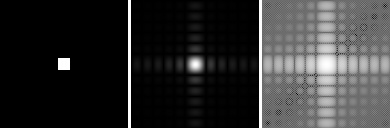
The images below are the DFT of both a circle or a square. The middle image is the DFT and the image at the far right is in log scale.


Apart from it being beautiful, The fourier transform of both these shapes can be associated with a plane wave hitting an aperture that share its spatial similarities. Hence, this an aperture can be thought of as a sort of optical fourier transform. The circle forms an airy pattern. This type of pattern is evident in telescopes or any optical element with a very small exit pupil. Most of the time, These patterns are unwanted in optical setups and are treated as aberrations or artifacts.
This was also done for the letter A. This will be used for the next part of the activity.

This goes to show that different images in real space corresponds to different patterns in the fourier domain.
Convolution
Convolution can be thought of as a multiplication of a two signals in the fourier domain. It is a sort of smearing of two functions in the real space. It is expressed as,
![]()
To help with the “smearing” i provide two gifs to show what a convolution does.


As you may have noticed, the circles are getting smaller! Wow! This may show that you are actually placing a pinhole over the lens. The Vip in the image plane (or in this case the fourier plane) becomes less and less sharp. This is due to the aberration given by the aperture size. (It shows a relative airy pattern on the edges of the VIP).
Not only did we learn about the property of the convolution but we also saw it’s potential in simulating optical systems! This is exciting because it can show the theoretical output for reference in experiments!
This is the code used for this part of the activity:
nx= 128 ; ny=128 ;

x = linspace(-1,1,128);
y = linspace(-1,1,128);

[X,Y] = ndgrid(x,y);

A = zeros(nx,ny);
side = .1
r = sqrt(X.^2 + Y.^2); // Circle

A(find(r<=1)) =1; //Circle radius

vip = imread('VIP.bmo location')

vip = rgb2gray(vip)
vip = double(vip)
fftvip = fft2(vip)

fftvip = uint8(255*log(abs(fftshift(fftvip)))/max(log(abs(fftshift(fftvip)))))

Fr = fftshift(A)
Fa = fft2(vip)

FRA = Fr.*Fa
IRA = fft2(FRA)
Fimage = abs(IRA)
final = uint8(255*Fimage/max(Fimage))
imshow(final)
Correlation
We can now know the “instances” so to speak of a signal because of the properties of both the fourier transform and the convolution thorem. Think of it this way, both signals are called to be similar if its correlation is equal to 1 and -1 if inversely similar. The range from -1 to 1 are considered to be the linear correlation of two signals. In this part of the activity we look into the correlation of a letter in a “jungle” of letters. I will show the results first before I continue with my elegant discussion.


The images above shows the process of determining the correlation of two distinct signals. The third image is the correlation of the two images. It shows where the letter “A” is located from the first image. The spots with the highest intensity shows that signal 2 has a high correlation value in that position thus giving away the position of the letter A in image 1. This is possible because information is stored in the fourier domain. If we know what information is being held by a signal, we can identify it with the other signals in the fourier space. Just like googling something in the internet.
This is the code i used for this part
rain=imread("image 1 location")

smalla=imread("image 2 location")

rain = double(rgb2gray(rain))
smalla = double(rgb2gray(smalla))

ftrain = fftshift(fft2(rain))

ftsmalla = fftshift(fft2(smalla))

mult = ftsmalla.*conj(ftrain)

mult = fftshift(fft2(mult))

mult = mat2gray(abs(mult))
imshow(mult)
This goes to show that the fourier domain contains a lot of information concerning real objects. This is the very reason why optical experiments are fun to do. There are still problems concerning the last part of the problem (although the problem may stem from the scilab interpreter ~sad face~). But the beauty that is these techniques knows no bounds. This is the foundation of one of the most used phase retrieval algorithms in optics (Gerchberg-Saxton). We all have our own fourier transforms. Til next time.
References:
[1] http://bmia.bmt.tue.nl/education/courses/fev/course/notebooks/Convolution.html
I will leave you with the fft of my lena. (This is only for fun)

As you may have noticed, facial structures contain very high frequencies. (Maganda kahit sa fourier space naks).

Leave a comment